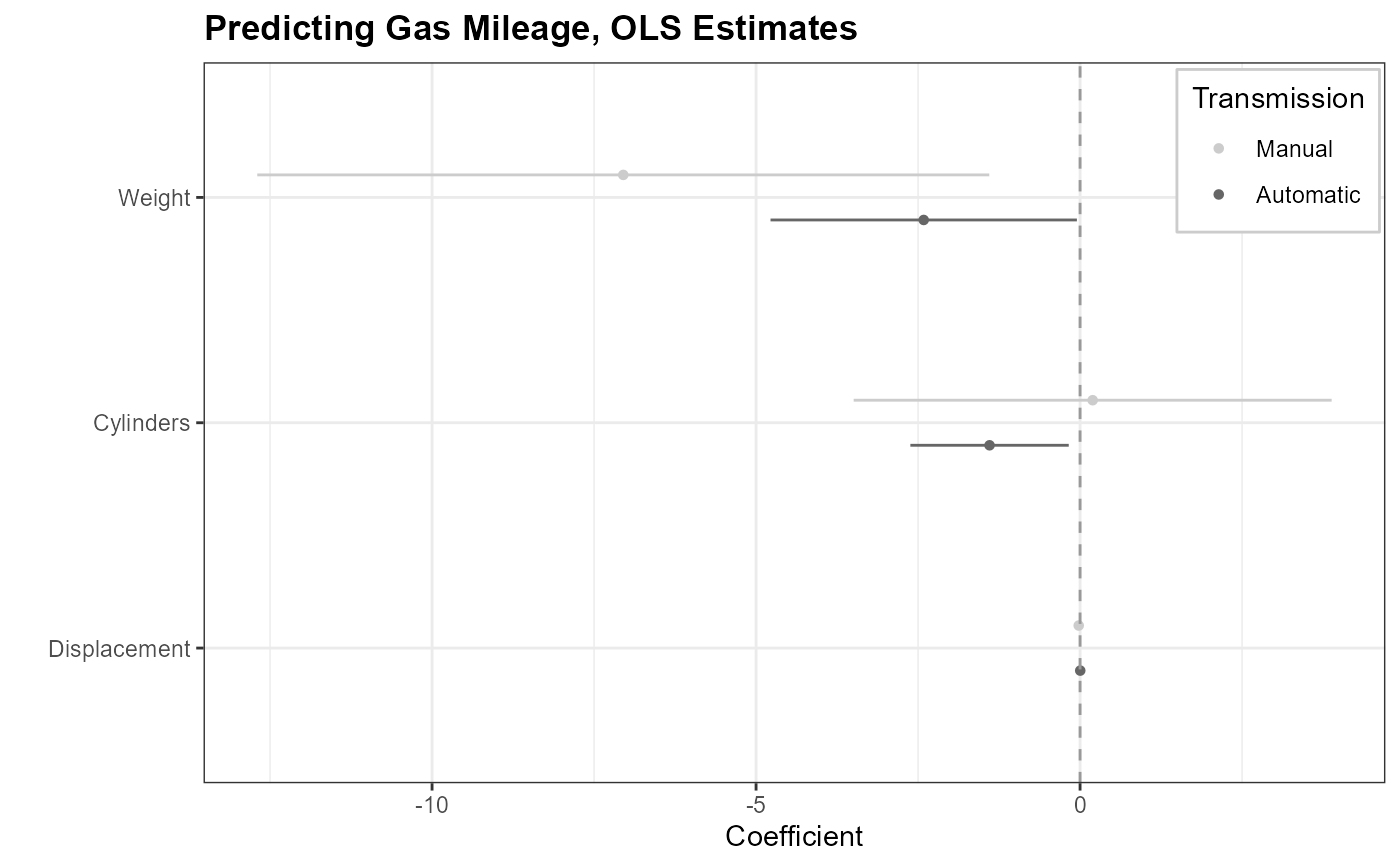
Dot-and-Whisker Plots of Regression Results

dwplot is a function for quickly and easily generating dot-and-whisker plots of regression models saved in tidy data frames.

dwplot(
  x,
  ci = 0.95,
  dodge_size = 0.4,
  vars_order = NULL,
  show_intercept = FALSE,
  show_stats = FALSE,
  stats_tb = NULL,
  stats_digits = 3,
  stats_compare = FALSE,
  stats_verbose = FALSE,
  stats_size = 10,
  stats_padding = unit(c(4, 4), "mm"),
  stats_layout = c(2, -1, 1),
  margins = FALSE,
  model_name = "model",
  model_order = NULL,
  style = c("dotwhisker", "distribution"),
  by_2sd = FALSE,
  vline = NULL,
  dot_args = list(size = 1.2),
  whisker_args = list(size = 0.5),
  dist_args = list(alpha = 0.5),
  line_args = list(alpha = 0.75, size = 1),
  ...
)

dw_plot(
  x,
  ci = 0.95,
  dodge_size = 0.4,
  vars_order = NULL,
  show_intercept = FALSE,
  show_stats = FALSE,
  stats_tb = NULL,
  stats_digits = 3,
  stats_compare = FALSE,
  stats_verbose = FALSE,
  stats_size = 10,
  stats_padding = unit(c(4, 4), "mm"),
  stats_layout = c(2, -1, 1),
  margins = FALSE,
  model_name = "model",
  model_order = NULL,
  style = c("dotwhisker", "distribution"),
  by_2sd = FALSE,
  vline = NULL,
  dot_args = list(size = 1.2),
  whisker_args = list(size = 0.5),
  dist_args = list(alpha = 0.5),
  line_args = list(alpha = 0.75, size = 1),
  ...
)

Arguments

x: Either a model object to be tidied with tidy, or a list of such model objects, or a tidy data frame of regression results (see 'Details').
ci: A number indicating the level of confidence intervals; the default is .95.
dodge_size: A number indicating how much vertical separation should be between different models' coefficients when multiple models are graphed in a single plot. Lower values tend to look better when the number of independent variables is small, while a higher value may be helpful when many models appear on the same plot; the default is 0.4.
vars_order: A vector of variable names that specifies the order in which the variables are to appear along the y-axis of the plot. Note that the order will be overwritten by relabel_predictors, if the function is following called.
show_intercept: A logical constant indicating whether the coefficient of the intercept term should be plotted. The default is FALSE.
show_stats: A logical constant indicating whether to show a table of model fitness statistics under the dot-whisker plot. The default is TRUE.
stats_tb: Customized table of model fit. The table should be in a data.frame.
stats_digits: A numeric value specifying the digits to display in the fitness table. This parameter is relevant only when show_stats = TRUE. Default is 3, providing a balance between precision and readability.
stats_compare: A logical constant to enable comparison of statistics in the fitness table. Applicable only when show_stats = TRUE. The default value is FALSE. That is, it presents all the statistics across different modeling methods, yet potentially expanding the table's breadth. When set to TRUE, only the shared, comparable statistics are remained.
stats_verbose: A logical constant to turn on/off the toggle warnings and messages of model fits. The default is FALSE.
stats_size: A numeric value determining the font size in the fitness table, effective only if show_stats = TRUE. The standard setting is 10.
stats_padding: Defining the internal margins of the fitness table. Relevant when show_stats = TRUE. Set by default to unit(c(4, 4), "mm"), allowing for a balanced layout. Further customization options refer to tableGrob.
stats_layout: Adjusting the spacing between the dotwhisker plot and the fitness table. Effective when show_stats = TRUE. The initial configuration is c(2, -1, 1), ensuring a coherent visual flow. Additional layout settings refer to plot_layout.
margins: [Suspended] A logical value indicating whether presenting the average marginal effects of the estimates. See the Details for more information.
model_name: The name of a variable that distinguishes separate models within a tidy data frame.
model_order: A character vector defining the order of the models when multiple models are involved.
style: Either "dotwhisker" or "distribution". "dotwhisker", the default, shows the regression coefficients' point estimates as dots with confidence interval whiskers. "distribution" shows the normal distribution with mean equal to the point estimate and standard deviation equal to the standard error, underscored with a confidence interval whisker.
by_2sd: When x is model object or list of model objects, should the coefficients for predictors that are not binary be rescaled by twice the standard deviation of these variables in the dataset analyzed, per Gelman (2008)? Defaults to FALSE. Note that when x is a tidy data frame, one can use by_2sd to rescale similarly.
vline: A geom_vline() object, typically with xintercept = 0, to be drawn behind the coefficients.
dot_args: When style is "dotwhisker", a list of arguments specifying the appearance of the dots representing mean estimates. For supported arguments, see geom_point.
whisker_args: When style is "dotwhisker", a list of arguments specifying the appearance of the whiskers representing the confidence intervals. For supported arguments, see geom_linerangeh.
dist_args: When style is "distribution", a list of arguments specifying the appearance of normally distributed regression estimates. For supported arguments, see geom_polygon.
line_args: When style is "distribution", a list of arguments specifying the appearance of the line marking the confidence interval beneath the normal distribution. For supported arguments, see geom_linerangeh.
...: Extra arguments to pass to parameters.

Value

The function returns a ggplot object.

Details

dwplot visualizes regression model objects or regression results saved in tidy data frames as dot-and-whisker plots generated by ggplot.

Tidy data frames to be plotted should include the variables term (names of predictors), estimate (corresponding estimates of coefficients or other quantities of interest), std.error (corresponding standard errors), and optionally model (when multiple models are desired on a single plot; a different name for this last variable may be specified using the model_name argument). In place of std.error one may substitute conf.low (the lower bounds of the confidence intervals of each estimate) and conf.high (the corresponding upper bounds).

For convenience, dwplot also accepts as input those model objects that can be tidied by tidy (or parameters (with proper formatting)), or a list of such model objects.

By default, the plot will display 95-percent confidence intervals. To display a different interval when passing a model object or objects, specify a ci argument. When passing a data frame of results, include the variables conf.low and conf.high describing the bounds of the desired interval.

Because the function can take a data frame as input, it is easily employed for a wide range of models, including those not supported by broom or parameters. And because the output is a ggplot object, it can easily be further customized with any additional arguments and layers supported by ggplot2. Together, these two features make dwplot extremely flexible.

dwplot provides an option to present the average marginal effect directly. Users can alter the confidence intervals of the margins through the ci argument. ^[The function is suspended due to the dependency issue. We'll work on getting it back in the next update.] The `margins` argument also works for small_multiple and secret_weapon.

To minimize the need for lengthy, distracting regression tables (often relegated to an appendix for dot-whisker plot users), dwplot incorporates optimal model fit statistics directly beneath the dot-whisker plots. These statistics are derived using the excellent performance functions and integrated at the plot's base via patchwork and tableGrob functions. For added flexibility, dwplot includes the stats_tb feature, allowing users to input customized statistics. Furthermore, a suite of stats_* functions is available for fine-tuning the presentation of these statistics, enhancing user control over the visual output.

References

Kastellec, Jonathan P. and Leoni, Eduardo L. 2007. "Using Graphs Instead of Tables in Political Science." *Perspectives on Politics*, 5(4):755-771.

Gelman, Andrew. 2008. "Scaling Regression Inputs by Dividing by Two Standard Deviations." *Statistics in Medicine*, 27:2865-2873.

Examples

library(dplyr)
# Plot regression coefficients from a single model object
data(mtcars)
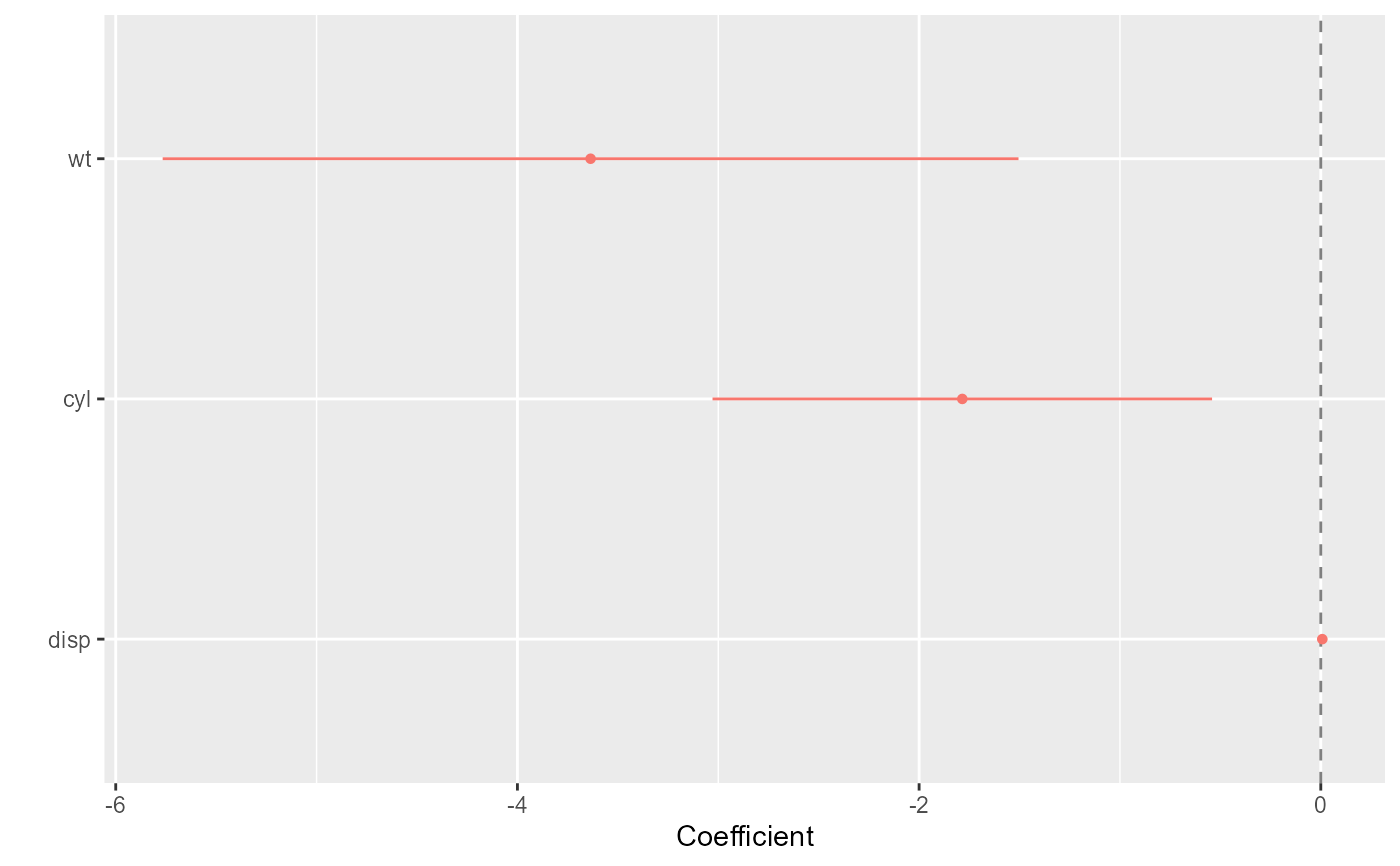
m1 <- lm(mpg ~ wt + cyl + disp, data = mtcars)
dwplot(m1, vline = geom_vline(xintercept = 0, colour = "grey50", linetype = 2)) +
    xlab("Coefficient")

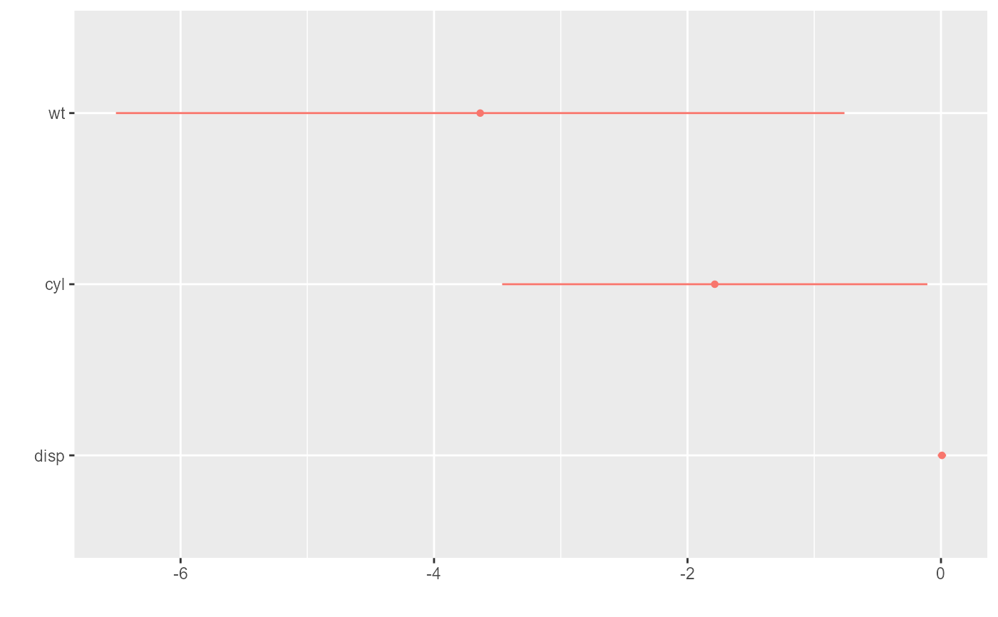
# using 99% confidence interval
dwplot(m1, ci = .99)

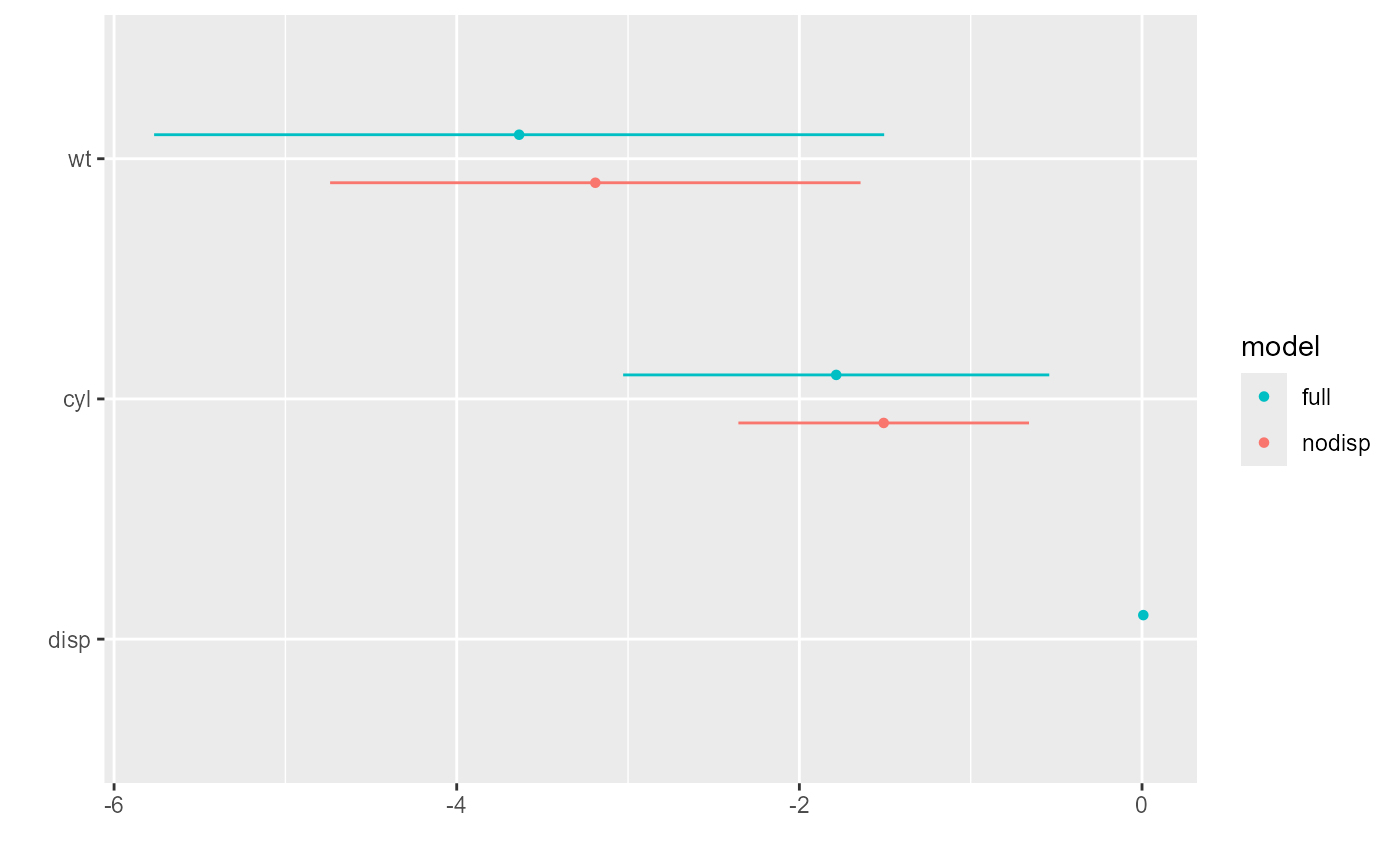
# Plot regression coefficients from multiple models
m2 <- update(m1, . ~ . - disp)
dwplot(list(full = m1, nodisp = m2))

# Change the appearance of dots and whiskers
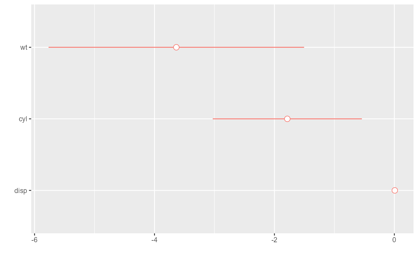
dwplot(m1, dot_args = list(size = 3, pch = 21, fill = "white"))

# Plot regression coefficients from multiple models on the fly
mtcars %>%
    split(.$am) %>%
    purrr::map(~ lm(mpg ~ wt + cyl + disp, data = .x)) %>%
    dwplot() %>%
    relabel_predictors(c(wt = "Weight", cyl = "Cylinders", disp = "Displacement")) +
    theme_bw() + xlab("Coefficient") + ylab("") +
    geom_vline(xintercept = 0, colour = "grey60", linetype = 2) +
    ggtitle("Predicting Gas Mileage, OLS Estimates") +
    theme(plot.title = element_text(face = "bold"),
          legend.position = c(.995, .99),
          legend.justification = c(1, 1),
          legend.background = element_rect(colour="grey80"),
          legend.title.align = .5) +
    scale_colour_grey(start = .4, end = .8,
                      name = "Transmission",
                      breaks = c("Model 0", "Model 1"),
                      labels = c("Automatic", "Manual"))
#> Warning: The `legend.title.align` argument of `theme()` is deprecated as of ggplot2
#> 3.5.0.
#> ℹ Please use theme(legend.title = element_text(hjust)) instead.
#> Warning: A numeric `legend.position` argument in `theme()` was deprecated in ggplot2
#> 3.5.0.
#> ℹ Please use the `legend.position.inside` argument of `theme()` instead.